Probability and tennis

The idea

The other day, while surfing Reddit, I came across a few comments that said having a 55% chance of winning a point would give you a 99% chance of winning the game. I’d heard this before, but this time I thought, “Hey! I can simulate that and see if it makes sense.” Seemed a bit unrealistic to me, that 50% would mean dead-even whereas 55% would mean a blowout.

Testing the “theory”

So, I went ahead and opened up python and wrote a little program to simulate a tennis match. I varied the probability of winning a point from 0.00 to 1.00, in steps of 0.01, and simulated 10000 matches for each probability. Matches were best of 5, with no tiebreaks - you had to be two games clear¹.

The results

Here are the results plotted in R:

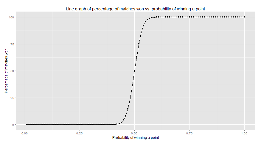
The line graph² shows that clearly there is a small range of probabilities where matches tend to be competitive. Examining the data, 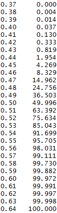we can see that this range varies from 0.38 to 0.63, or 0.15 above and below a 50% chance to win a point. All values below 0.38 led to all matches being lost and all values above 0.63 lead to all matches being won. The data also shows that having a probability of around 0.57 of winning a point (slightly higher than what I’d seen on Reddit) would give you a 99% chance to win the match.

Further investigation

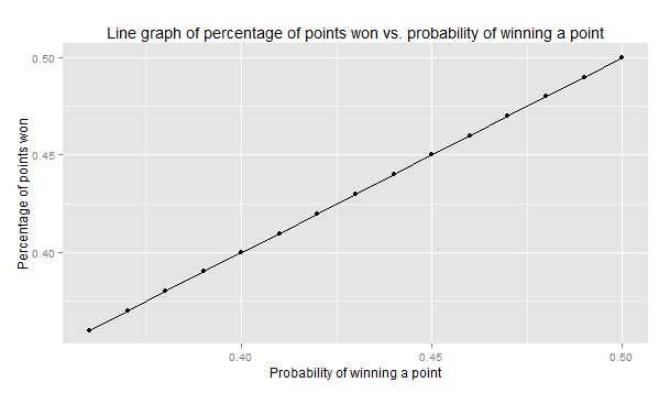
To use this information, we need to estimate the probability of winning a point. This can be done by taking the percentage of points won from previous matches and using that as the probability. Is that a reasonable assumption? To verify, I used the data from the simulations I ran earlier. A straight line at a 45-degree angle would indicate that this was a reasonable assumption. Since the range of interest for probabilities was between 0.38 to 0.50, I re-ran the simulations in that - smaller - range (python is slow). Thankfully, the data agreed:

Now, all that was left was to put this to use. I figured in most head-to-heads, both players woud have similar total points won. This would mean that the ratio of points won falls in the expected range (0.38 to 0.63). An interesting matchup to look at would be one with one player having a dominant head-to-head losing the match. Nadal-Wawrinka have a head-to-head of the second type.

Nadal-Wawrinka’s points won are: matches = [(99,62),(80,71),(69,55),(97,89),(59,48),(82,75),(63,51),(73,58),(59,39),(96,64),(75,59),(80,83),(88,116),(75,81)]

Considering Wawrinka was able to beat Nadal after losing to him 12 times straight, Nadal’s points won ratio should ideally not be at or above 0.57 and not below 0.52. Over all except the last two matches (the only ones Wawrinka won), Nadal has a points won ratio of 0.5528. This would give him a 96% chance of winning. With all matches considered, his points won ratio is at 0.5352, around 85% chance of winning a match. Their head-to-head stands at 85.7% matches won by Nadal.

As a final task, I calculated the theoretical minimum points won ratio that could win a match:

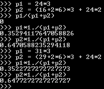
This would occur when the loser wins 2 sets 6-0 and goes either 6-4 (without tiebreaks) or 6-6 (5) in the other 3 sets, while winning 2 points in each game the winner wins. The first half shows the ratios without tie-breaks, the second one considers a match with tiebreaks. The minimum points won ratio is 0.3529, and this scenario is rare enough that it didn’t occur even once in 10000 simulations.

Codebook

Python program for simulating tennis matches

import random 

class Match:
    def __init__(self, sets_to_win):
        self.to_win = sets_to_win
        self.player1 = []
        self.player2 = []
        self.curr_game = [0,0]
        self.games = [0,0]
        self.sets = [0,0]

    def update(self, pointTo):
        self.curr_game[pointTo] += 1
        if (self.curr_game[pointTo] > 3 and self.curr_game[(pointTo+1)%2] < self.curr_game[pointTo] - 1):
            self.games[pointTo]+=1
            self.curr_game = [0,0]
        if self.games[pointTo] > 5 and self.games[(pointTo+1)%2] < self.games[pointTo] - 1:
            self.sets[pointTo] += 1
            # Uncomment to see the match results
            # print self.games
            self.games = [0,0]

    def Over(self):
        return max(self.sets[0],self.sets[1]) >= self.to_win

    def Winner(self):
        return 0 if self.sets[0] > self.sets[1] else 1

def playPoint(threshhold):
    return 0 if random.random() > threshhold else 1

def playMatch(prob):
    match = Match(3)
    points = [0,0]
    while not match.Over():
        pointTo = playPoint(prob)
        match.update(pointTo)
        points[pointTo] += 1
#    Percentage of points won by each player
#    if points[match.Over()-1] < points[match.Over()%2]:
#        print points[0]*1./(points[0] + points[1])
#        print points[1]*1./(points[0] + points[1])
#        print match.Over()
    return match.Winner()

if __name__ == "__main__":
    for prob in xrange(0,101):
        wins = [0,0]
        for _ in xrange(0,100000):
            wins[playMatch(prob/100.)] += 1
        print prob/100., ", ",wins[0], ", ", wins[1]

R program to generate the plot

install.packages("ggplot2")
library(ggplot2)

prob = read.csv("tennisoutput.csv")

## Remove matches lost - Cleaning data
prob[,2] = NULL

## Change matches won to percentage of matches won
prob[,2] = prob[,2]/1000.00

## Assign column names
names(prob)[1] <- "PointProb"
names(prob)[2] <- "MatchProb"

ggplot(data=prob,aes(x=PointProb, y=MatchProb)) + geom_line() + geom_point() + xlab("Probability of winning a point") + ylab("Percentage of matches won") + ggtitle("Line graph of percentage of matches won vs. probability of winning a point") + geom_text(aes(label=ifelse(PointProb==0.57,paste(PointProb,MatchProb,sep=", "),'')),hjust = 0, size = 3, vjust = 1.4, colour = "brown")

Appendix

Someone did the math on this. I haven’t verified it, but you can read it here.